Introduction to Reinforcement Learning

December 3, 2022

Reinforcement Learning

⊕
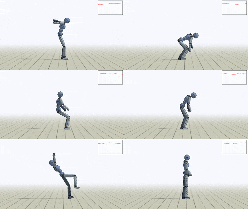
An example of reinforcement learning: the agent learns optimally to backflip.
Source: Composing Value Functions in Reinforcement Learning

In this blogpost we will introduce the most important concepts in Reinforcement learning and provide some real world examples, to show you how and when it is currently being used.

This series is based on the lectures that DeepMind held for UCL in 2020, they are freely available at this YouTube link.
I suggest you to watch these videos because they are extremely clear in my opinion. I chose to write this series of blogposts to offer a readable format of the content of DeepMind’s lectures.

Introduction

Reinforcement Learning is the branch of Computer Science that studies how to learn to perform tasks by modeling them as the maximization of a reward obtained by interacting with an environment.

This interaction can be summarized in the following diagram:

⊕
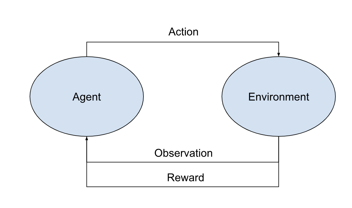
Reinforcement Learning entities diagram

Let’s describe it, introducing right away some terminology:

• Agent
  The computer system whose goal is to maximize a reward
• Environment
  The system the agent interacts with (by performing actions) and learns from (by observing changes in the environment’s state and collecting rewards)
• Reward \((R_t)\)
  a scalar feedback signal that indicates how well the agent is doing at timestep \(t\).

Shortly, at each timestep \(t\) the agent

• receives from the environment an observation \(O_t\)
• receives a reward \(R_t\)
• executes an action \(A_t\)

This was a very high level description of the core entities involved in the reinforcement learning problem. But what is it used in? Here are some examples:

• Fly a helicopter
• Manage an investment portfolio
• Control a power station
• Make a robot walk
• Play video or board games

Now let’s delve into a lower level description, where I will introduce the mathematical terminology that will be used throughout the next episodes.

The Environment

It is a system in which you can perform actions and, consequently, it will

• change its state
• give you a reward

This type of system is modeled as a Markov decision process, namely a mathematical framework that models decision making problems.
Look at the image below. It represents a graph with three nodes \((S_0, S_1, S_2)\).
From each state you can perform some actions that will lead you to another state with a certain probability. We associate a reward (the orange arrows) to some of these actions.

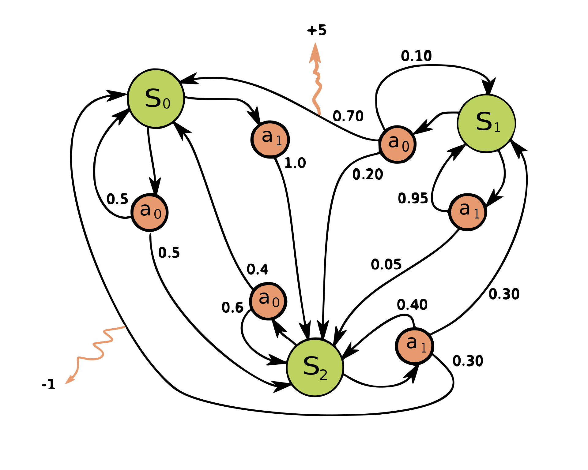
Rigorously, a Markov Decision Process is defined as a

• a set of states \(S\) called the set space
• a set of actions \(A\) called the action space
• a transition probability distribution
  \(P(s'|s_t,a_t): S\times A \to S\) that tells you what is the probability to go to state \(s'\) if you perform action \(a_t\) in state \(s_t\).
• A reward function \(R(s_t, a_t, s'):S \times A \times S \to \mathbb{R}\) that returns a scalar feedback (an immediate reward) when you perform action \(a_t\) in state \(s_t\) and end up in state \(s'\).

Moreover, the transition probability distribution \(P\) must satisfy the Markov property:

This means that

1. the state \(s'\) into which we transition after performing action \(a_t\) from state \(s_t\)
2. the obtained reward \(r\)

are independent from the history of the game (namely, the sequence of actions, observations, and rewards obtained so far).

In other words, \(s_t\) contains all the information we need to choose what action to perform next.

We have described extensively how we model an environment in Reinforcement Learning. It’s important though to note that the agent could have full knowledge about the environment state or not.

• Fully observable environment

  The environment is fully observable if \(S_t = O_t = \text{environment state}\) This means that the agent’s state is equivalent to the environment’s state.

• Partially observable environment
  An environment is partially observarble if the observations are not Markovian.
  The environment state can still be Markovian, but the agent does not know it.

  In this case the agent state is a function of the history.

  For instance \(S_t=O_t\), more generally:

  \[S_{t+1}=u(S_t, A_t, R_{t+1}, O_{t+1})\]

  The agent state is often much smaller the environment state.

An example of Partially Observable Environment

Imagine you are looking at a maze from above.

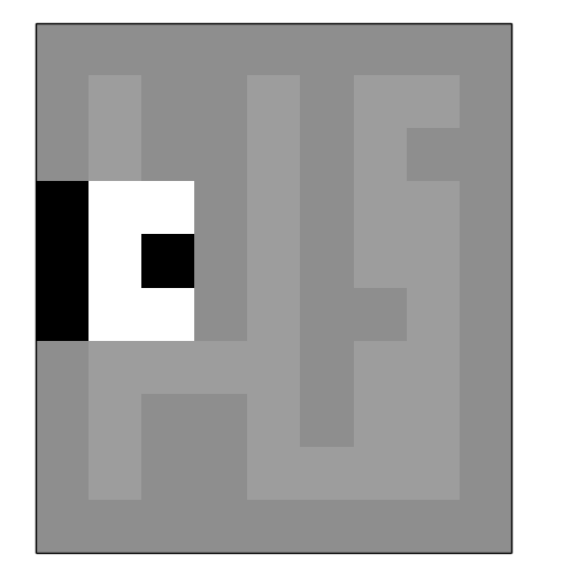
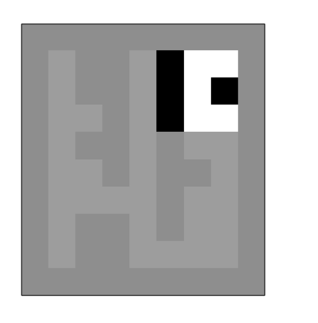
These two agent states are not Markovian because the only way we have to understand whether we are on the left side or the right side of the labyrinth is to analyze the agent’s history, checking what was the observation at previous timesteps.

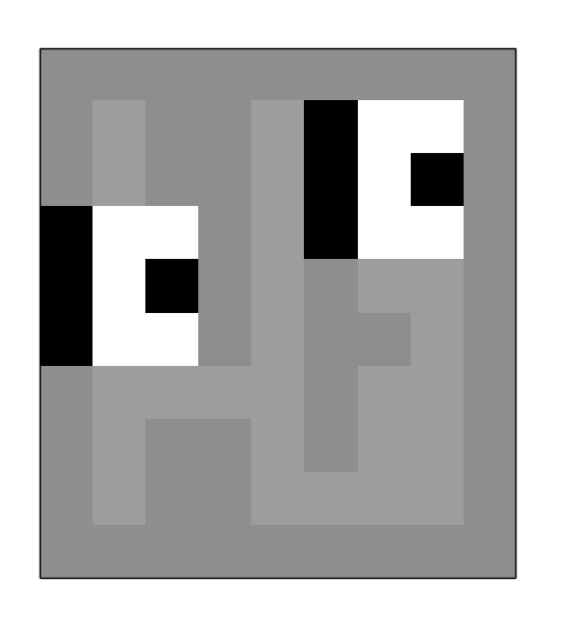
You could not construct a Markov agent state in this maze.

To deal with partial observability, an agent can construct a suitable state representation \(\to\) this is when the concepts of value function and action value function come in handy.

The Value Function

The value function is a function \(v(s): S \to \mathbb{R}\) that returns for each state \(s \in S\) the expected cumulative reward the agent will get by finding himself in such state.

The Policy

A policy is a function \(\pi: S \to A\) that, given a state \(s\), tells the agent what is the optimal action \(a\) to perform (the optimal action is the one that will lead him to the state with the highest expected cumulative reward).
A policy can be deterministic (the state-action mapping is univoque) or stochastic. In this latter case you will get in output a probability distribution over the actions set \(A\).

The Q value

A function that maps a state action pair \((s, a)\) to the expected cumulative reward.

That’s all for this introductory blogpost! See you in the next one.